Using Deep Learning to Better Detect Command Obfuscation

Author: Wilson Tang, Machine Learning Security Engineer Intern

Command obfuscation is a technique to make a piece of standard code intentionally difficult to read, but still execute the same functionality as the standard code. For example, look at these two code snippets:

When executed, they do the exact same thing. Crazy, right?

Malicious attackers can use obfuscation to make their malware evade traditional malware detection techniques, since attackers can create a virtually infinite number of ways to obfuscate their malware.

Because traditional malware detection techniques are typically rule-based, they are inflexible to new types of malware and obfuscation techniques. One way to detect these obfuscations is through deep learning, creating models that are dynamic and can adapt to new types of information.

The Security Intelligence team at Adobe, which is part of the company’s Security Coordination Center (SCC), decided to apply deep learning techniques to increase our ability to detect command obfuscation, thereby helping to improve overall security. We’ve open-sourced the results of the project so you can check it out yourself after reading this blog. The full code can be found on https://github.com/adobe/SI-Obfuscation-Detection.

Now, onto the rest of the blog:

Command obfuscation can’t be that bad, can it?

Well, let me tell you, it can be that bad. One method to detect malware on computers is to log and analyze all system commands that are being executed, hoping to detect anything that is out of place. For example, you open a document from a convincing phishing e-mail, the document executes some obfuscated system commands and wham! Your malware detection software can’t detect the obfuscation. In this situation, there’s a strong chance you won’t know that anything is wrong with your computer. Why? Let me explain:

Let’s say the term “cmd.exe” is a malicious command (it isn’t, but we’ll say it is for the sake of simplicity). One way to detect this malicious command is to monitor whether “cmd.exe” occurs inside any system command executed on your computer. And when we detect this term, we can raise a flag on the computer and act appropriately. This is rule-based detection.

However, command obfuscation renders rule-based detection useless. It’s easy to obfuscate the command “cmd.exe” into “cm%windir:~ -4, -3%.e^Xe”. This obfuscated term means the same thing as “cmd.exe” to the computer but can now evade the “cmd.exe” rule. And since an infinite number of ways exist to obfuscate “cmd.exe,” capturing all the possibilities with strict rule-based semantics is nearly impossible.

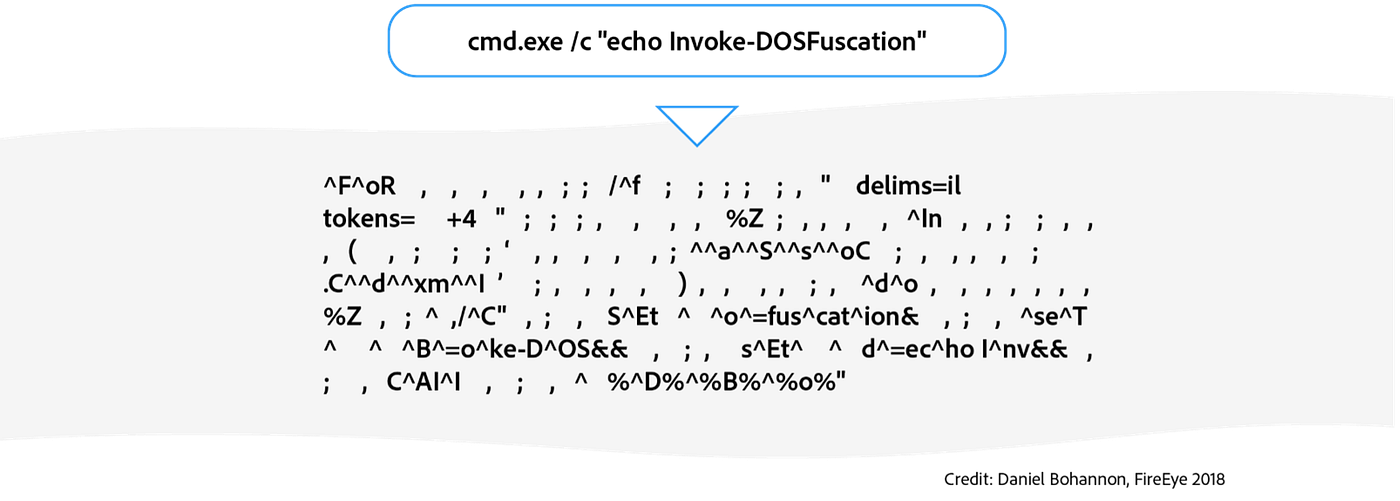
As the animation below shows, a single command can be altered with many layers of obfuscation. Each intermediate layer still means the same thing as the original command, showing the many ways the same command can be obfuscated.

Deep Learning to the Rescue!

There are several ways to detect command line obfuscation. Basic methods refer to statistics applied over known/unknown words (tokens) ratios and simple n-gram based language models. However, with the right amount of data, deep learning has been shown to outperform traditional natural language processing (NLP) methods on classical mainstream tasks.

As we found in our experiments, deep learning is also able to provide a robust solution of detecting obfuscated command lines. Intuitively, this is because command obfuscation can take many different forms and deep learning excels at creating models that are more dynamic and perform better on previously unseen data than traditional machine learning techniques.

Our model is a character-level deep convolutional neural network (CNN) — and that’s not a cable network.

Let’s break it down by each component:

Character level

We represent each command as a series of characters. In many NLP tasks, it is common to represent the data by each word. But because of the inconsistent syntax of obfuscated and non-obfuscated commands and for a higher level of granularity, we chose to represent our data by the character level.

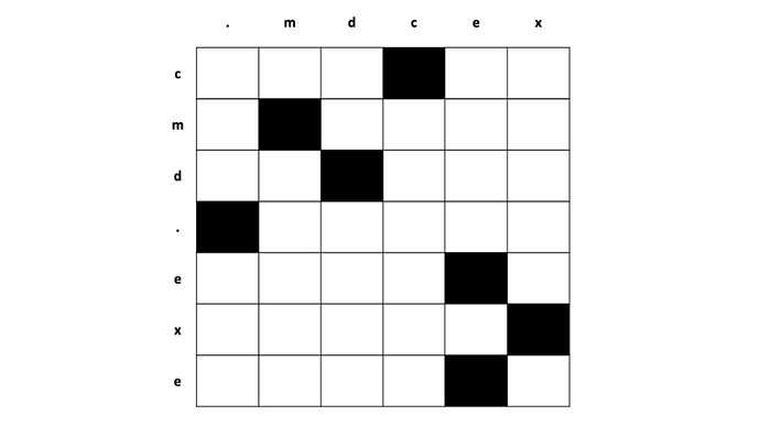
Each character in a command is represented by a one-hot vector, a vector where all the values are 0 except for the one index that represents which character it is in the string. We also include an extra case bit to differentiate between uppercase and lowercase characters. We found 73 characters as the most common character in our dataset. With the case bit, each character one-hot vector is 74-dimensional. Each command is also represented by its first 4096 characters. If the command is longer than 4096 characters, the rest is cut off and if the command is shorter, then the rest is padded with zeroes.

Therefore, the input to our model is a 74x4096 matrix:

Convolutional Neural Network (CNN)

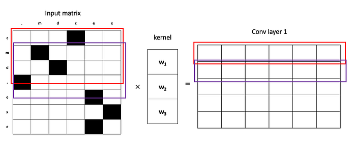
Traditionally, CNN’s have been used for computer vision tasks, e.g., images. This is because of the human observation that neighboring pixels in an image are closely related to each other. The same observation holds true here: neighboring characters are related to each other. So, for one convolutional layer (conv layer), we take a few neighboring characters (3 for our example), multiply them by some weights, and output a one-dimensional vector. This vector now carries semantic meaning for the first three characters (outlined by the red box).

Deep

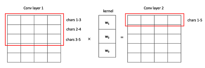
Now that was one conv layer. The “deep” part in this model is that we have many layers stacked on top of each other. The first conv layer now contains a matrix of vectors, where each row carries the semantic meaning of three characters. We continue this process of applying convolutions, thereby increasing the “window size” seen by each row in the matrix. If we apply one more layer of convolutions to our example, the next conv layer (conv layer 2) will contain rows where each row carries the semantic meaning of five (5) characters. The higher the layer, the bigger its window size. The bigger the window size, the more semantic meaning each row the conv layer can carry.

We continue this process of applying conv layers to each subsequent layer to extract meaning from the command as a whole. This process is known as feature extraction. After all our conv layers are applied, we finally make a decision by taking an average of the CNN’s output (final layer). This average is then run through a final fully connected (FC) layer to make the final output. Here is an animation of our full model:

Results

F1 score is a metric typically used to measure how well the model is doing. The score ranges from 0 to 1. Accuracy is another common metric, but because our dataset is imbalanced, accuracy is an unreliable metric. F1 score is preferred for imbalanced datasets.

With our dataset and model, we achieved an f1 score of 0.9891! The root cause of our remaining small errors is small mistakes on false negatives, classifying commands as not obfuscated when they are obfuscated. These cases are from commands that are very slightly obfuscated. We have also improved on previous work by FireEye in 2017, which this project was built upon (source). They stated an f1 score of 0.95 with their own model and dataset.

Overall, this project can be easily applied to other use cases, such as malware detection and phishing detection. We have published a public pip package at https://pypi.org/project/obfuscation-detection/ with documentation on how to use our model easily in your own Python projects.